Convectively Coupled Tropical Waves (CCEWs)
Codes by Sandro W. Lubis
(Former) Master Student at the Institute of Meteorology, University of Leipzig, Leipzig, Germany, 2015
and (Former) Ph.D. Student at the GEOMAR – Helmholtz Centre for Ocean Research Kiel, Kiel, Germany, 2018
Updated: May, 2022
Related Works !!:
- Lubis, S. W., and Respati, M. R. (2020). Impacts of Convectively Coupled Equatorial Waves on Rainfall Extremes in Java, Indonesia. International Journal of Climatology 41, 4, 2418-2440. Link.
- Lubis, S. W., and Jacobi, C. (2015). The Modulating Influence of Convectively Coupled Equatorial Waves (CCEWs) on the Variability of Tropical Precipitation. International Journal of Climatology 35, 7, 1465-1483. Link.
Attention !!:
This blog was designed under Linux operating system thus I apologize this page will not look nice if you are using another operating system.
=======
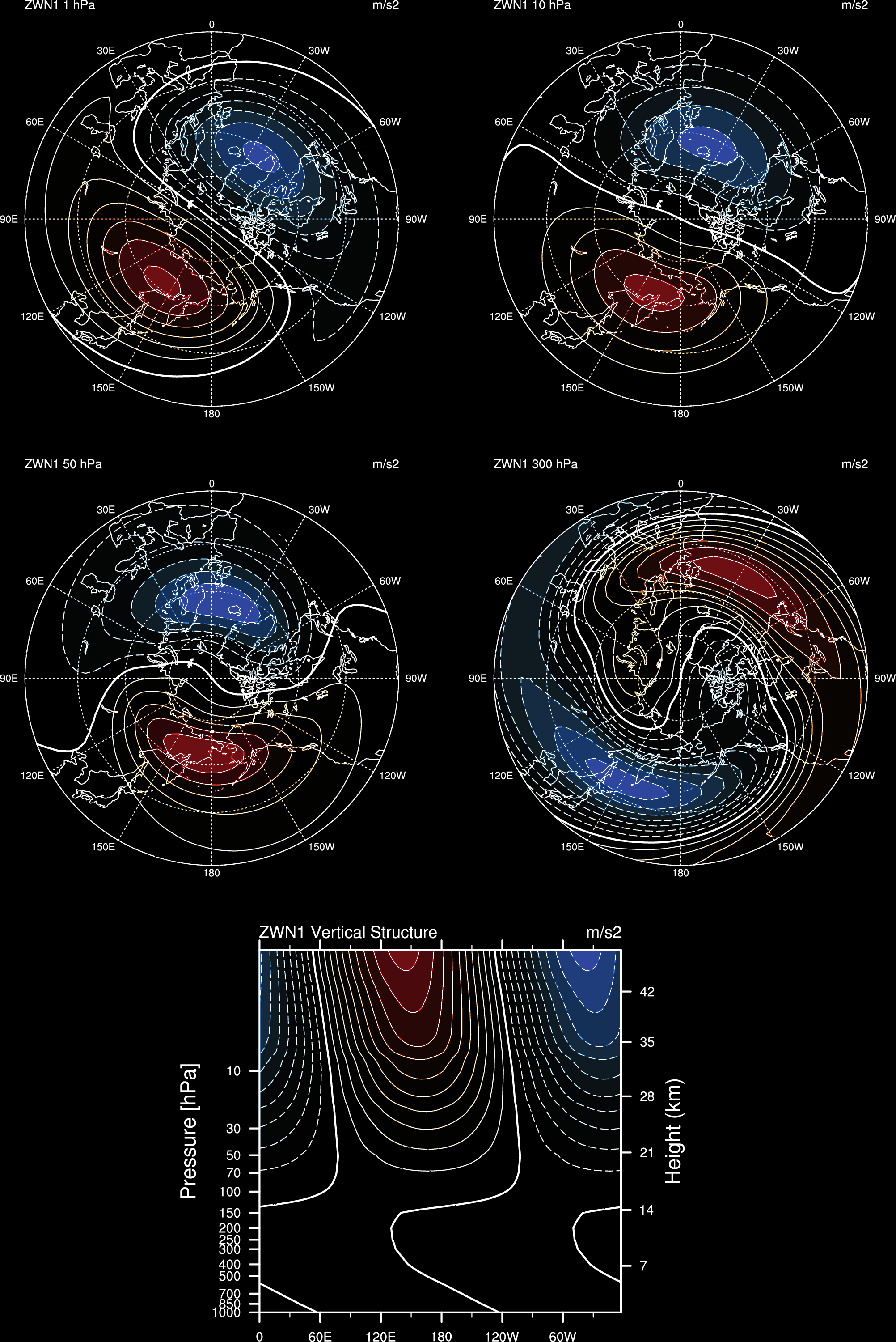
“Forced Stationary Waves”
======================================
Theoretical structure of atmospheric forced stationary waves in the tropics. The heating response Q is the forcing term which is proportional to the vertical derivative of the diabatic heating and the dissipation rate (representing Rayleigh friction), and Newtonian cooling is assumed to 0.2 (nondim). The background atmosphere was assumed to be at rest. Once the set of forcing functions for u, v and 
—

====
“Free Equatorial Waves”
======================================
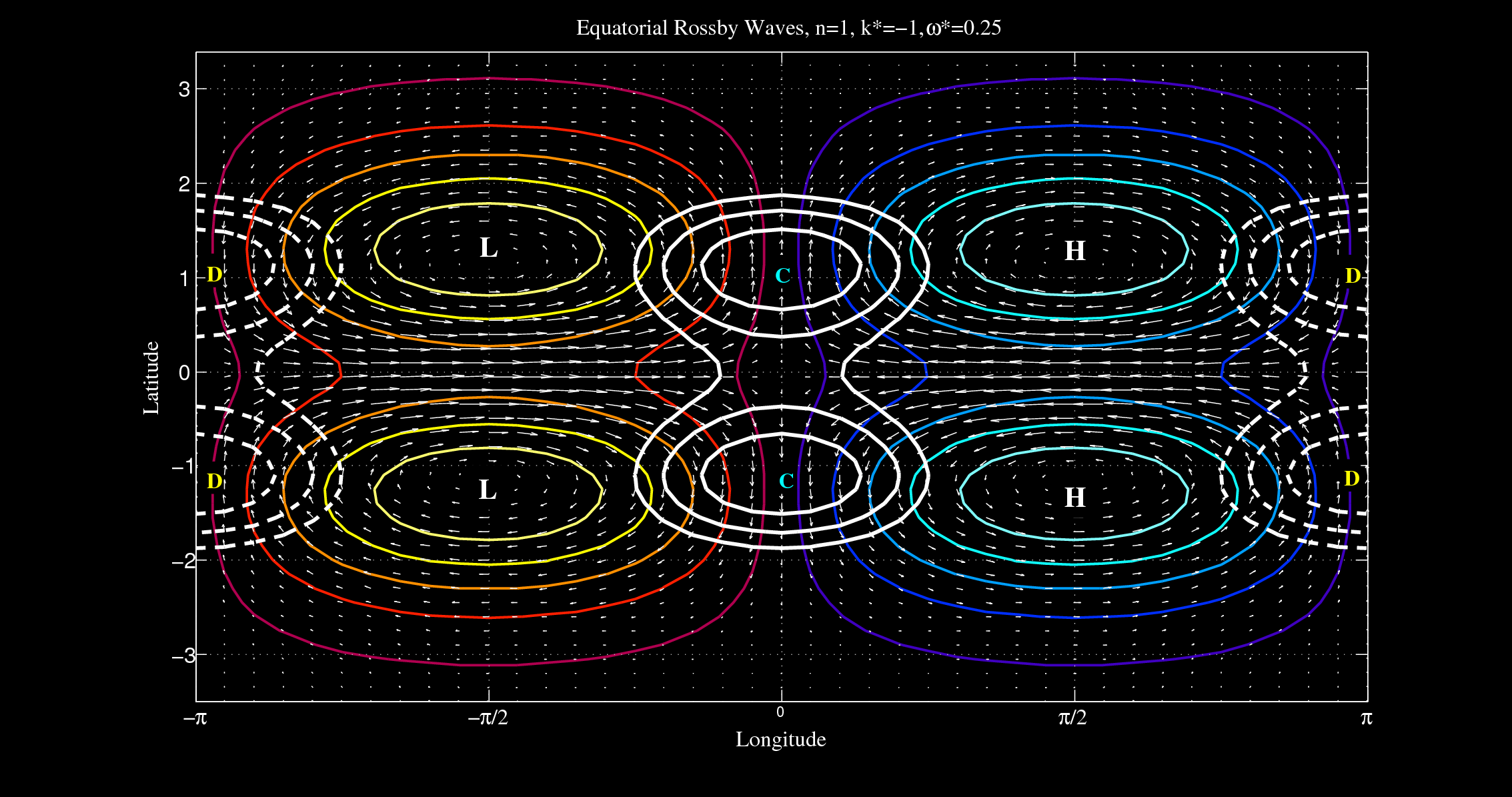
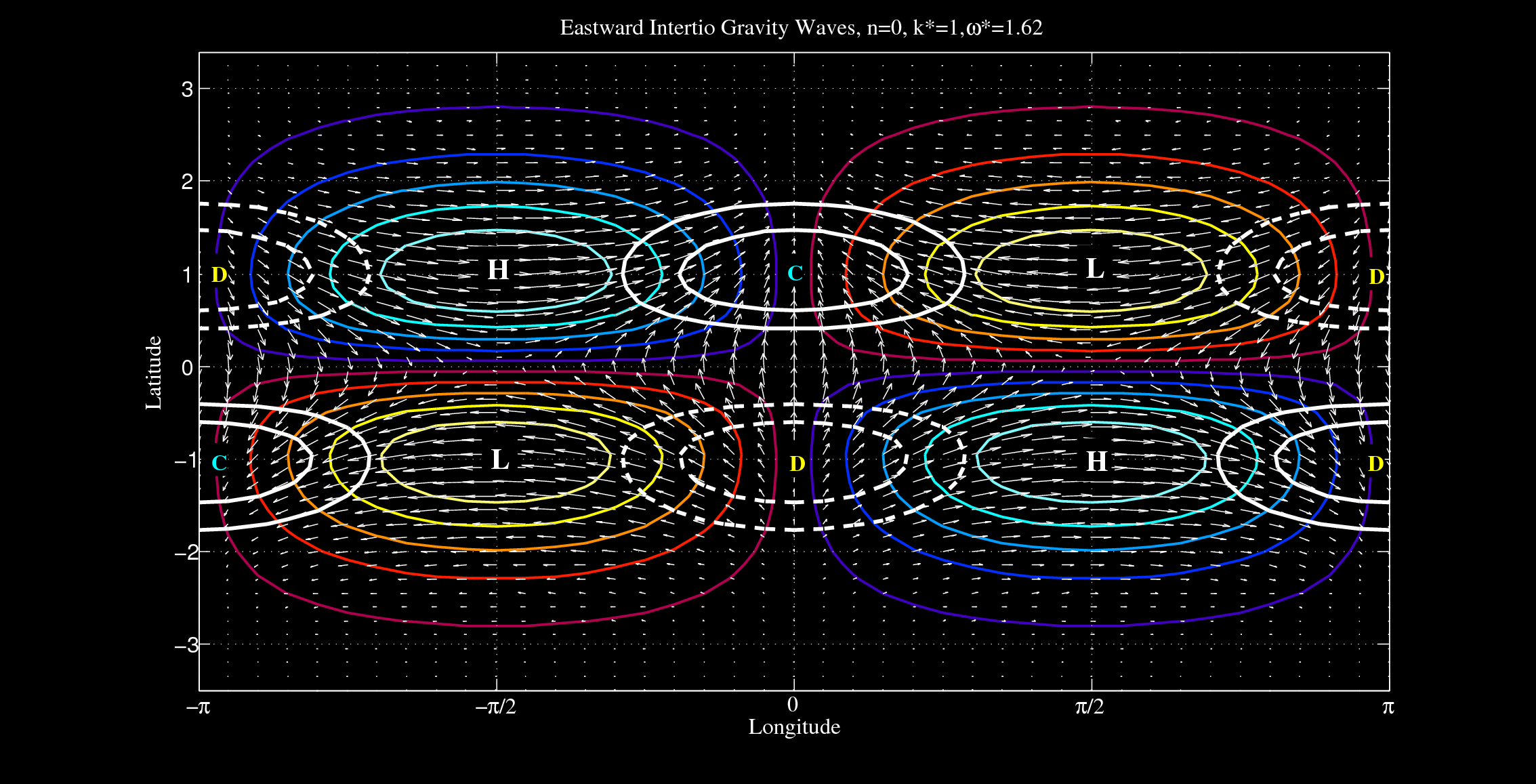
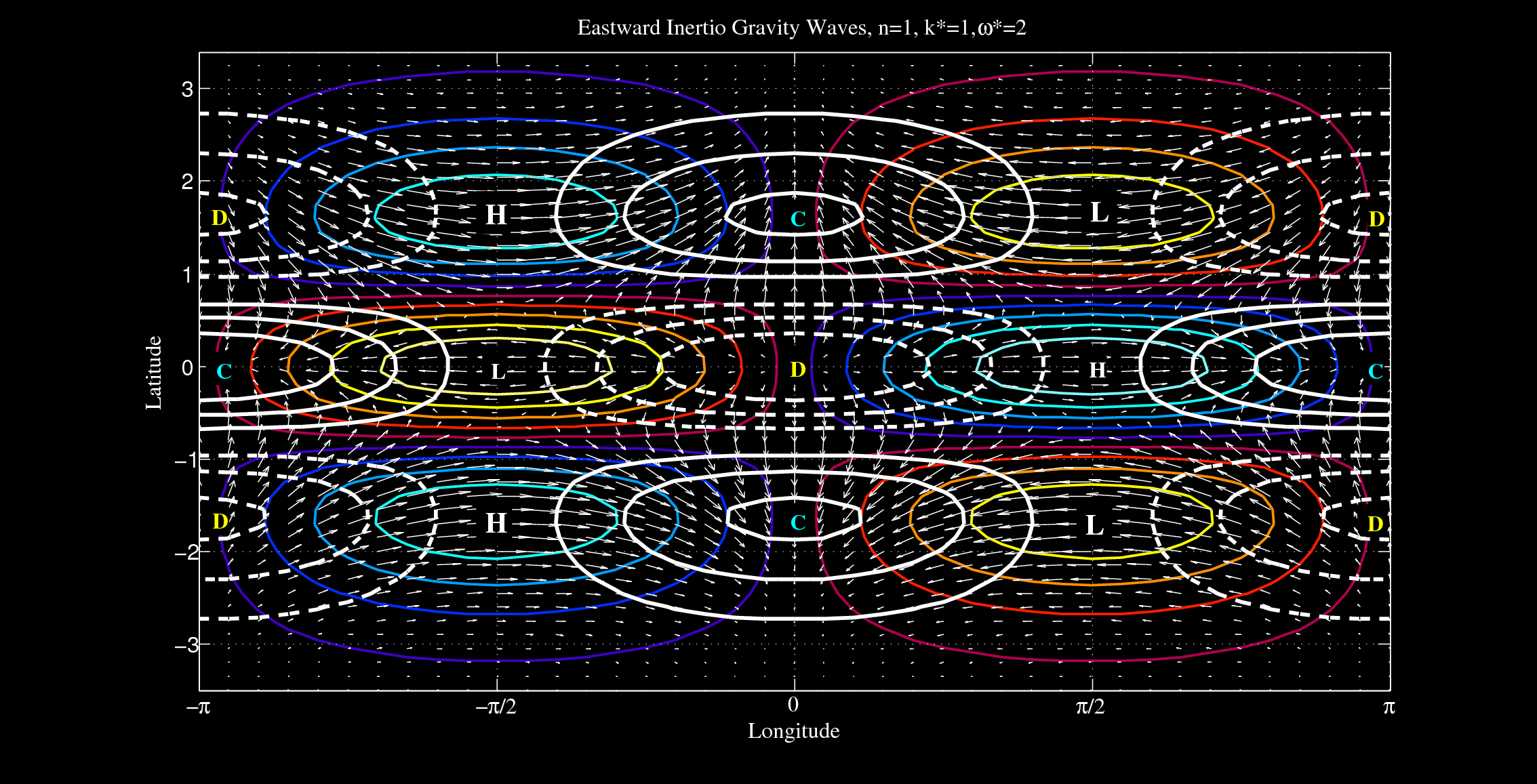
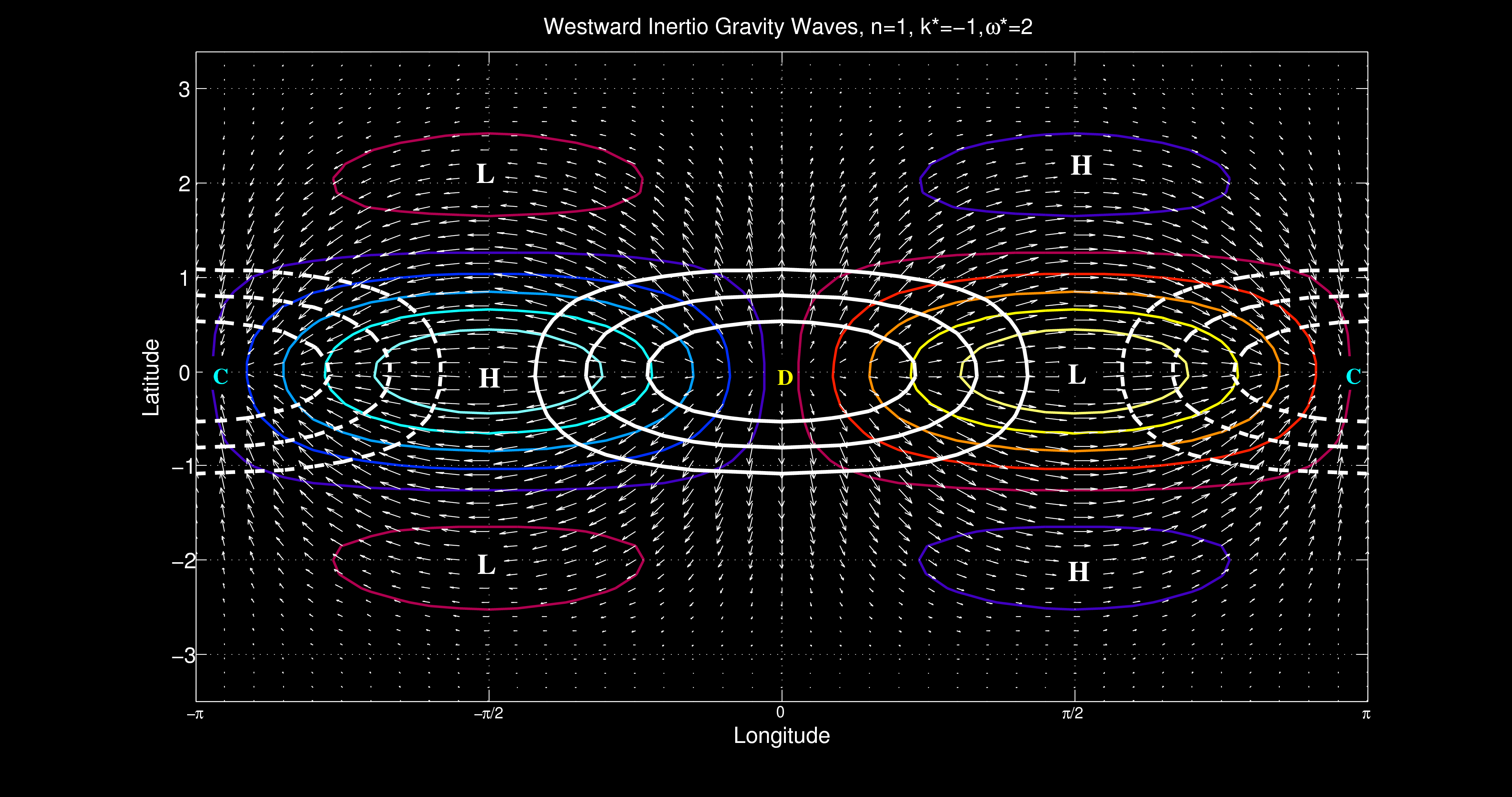
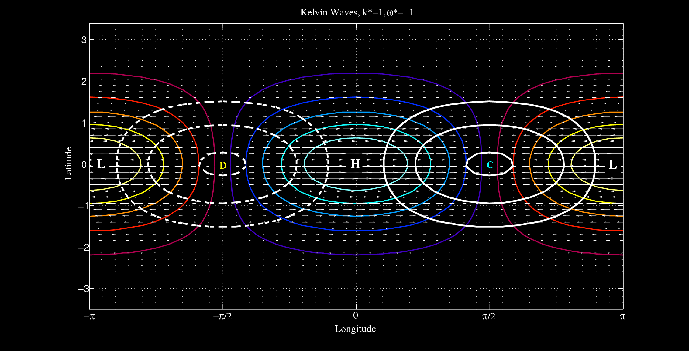
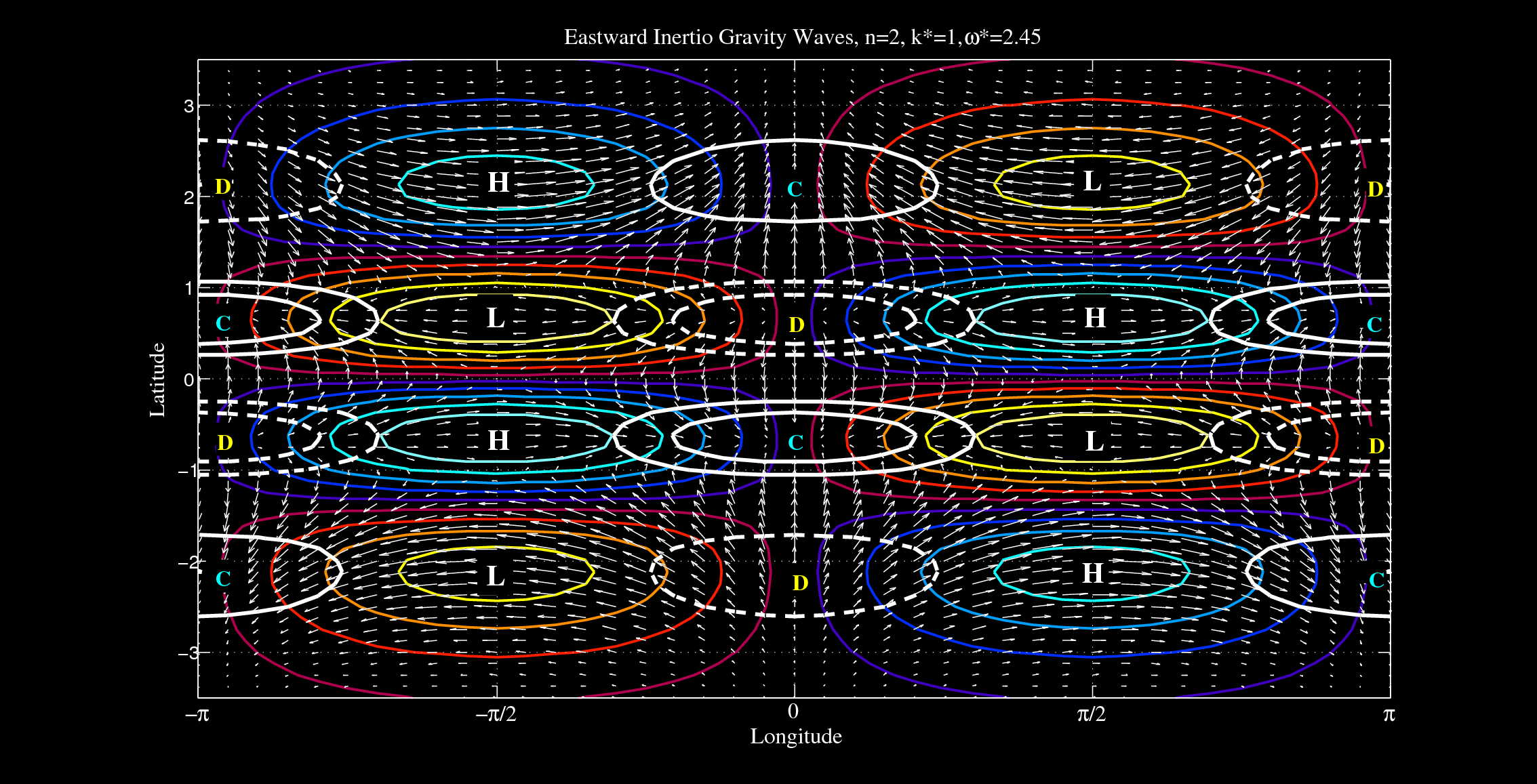
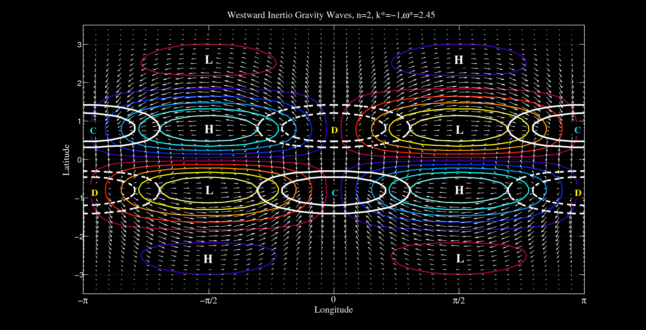
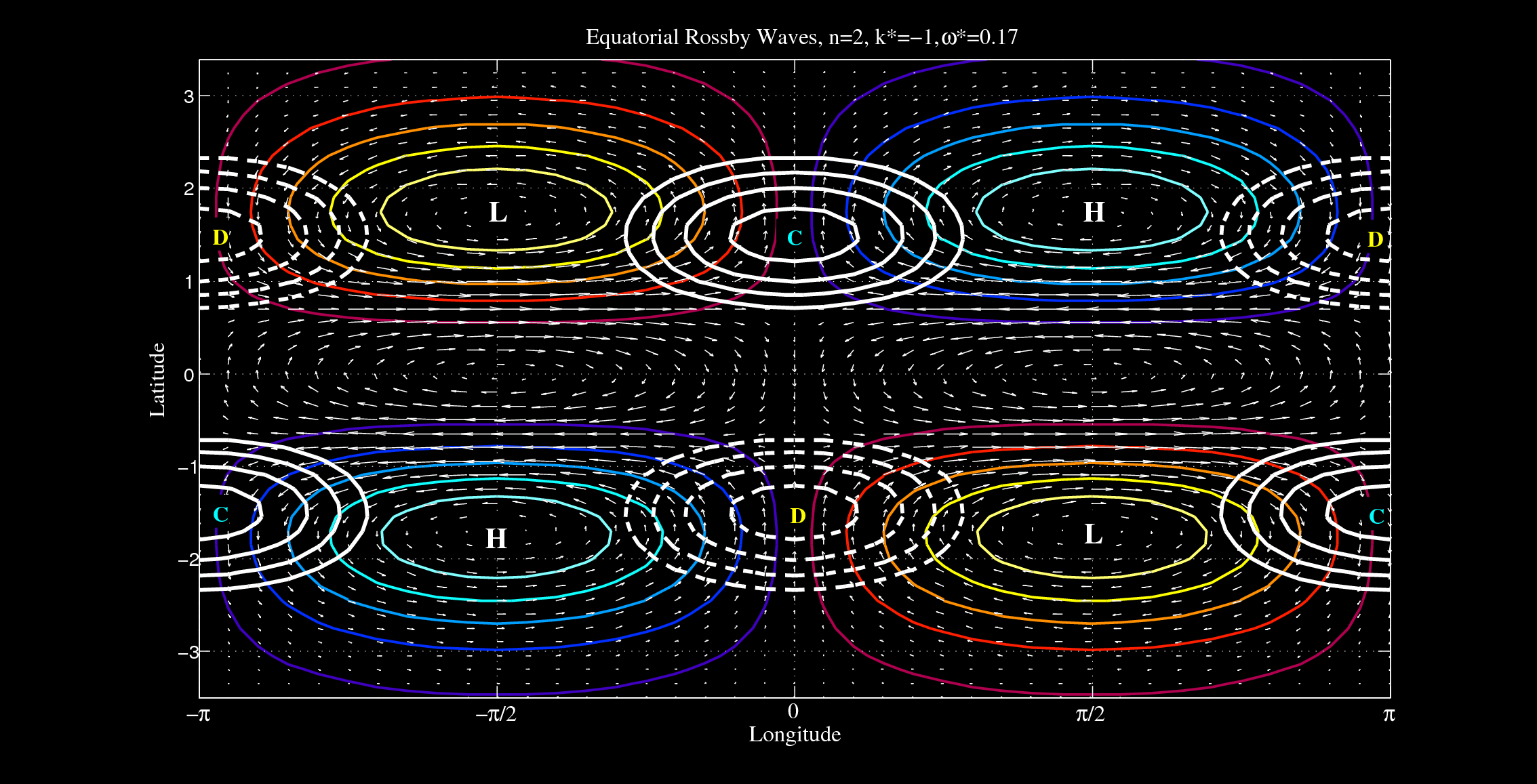
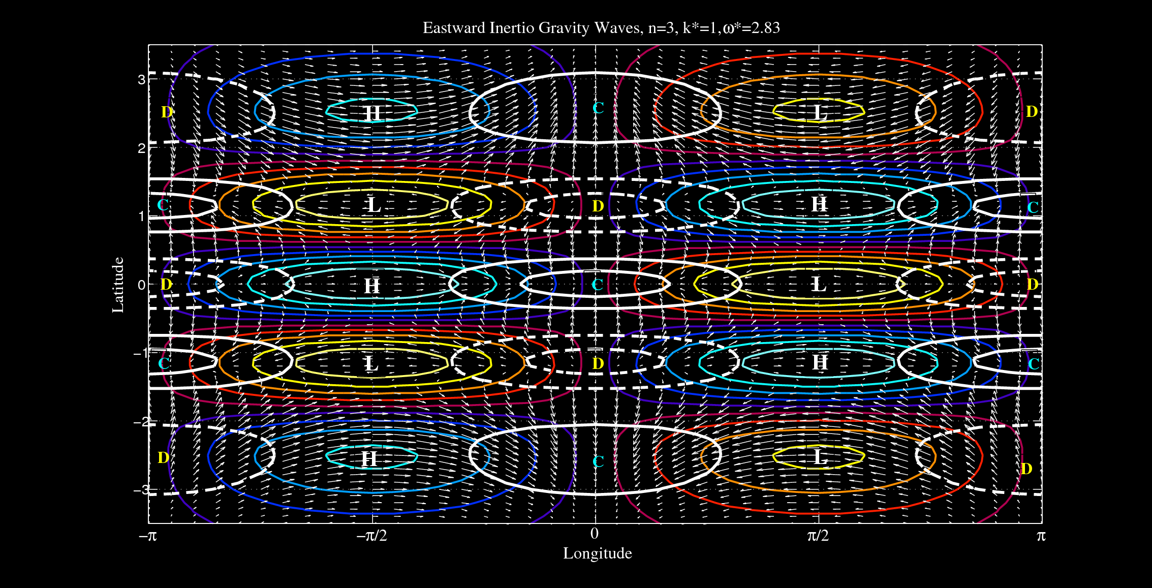
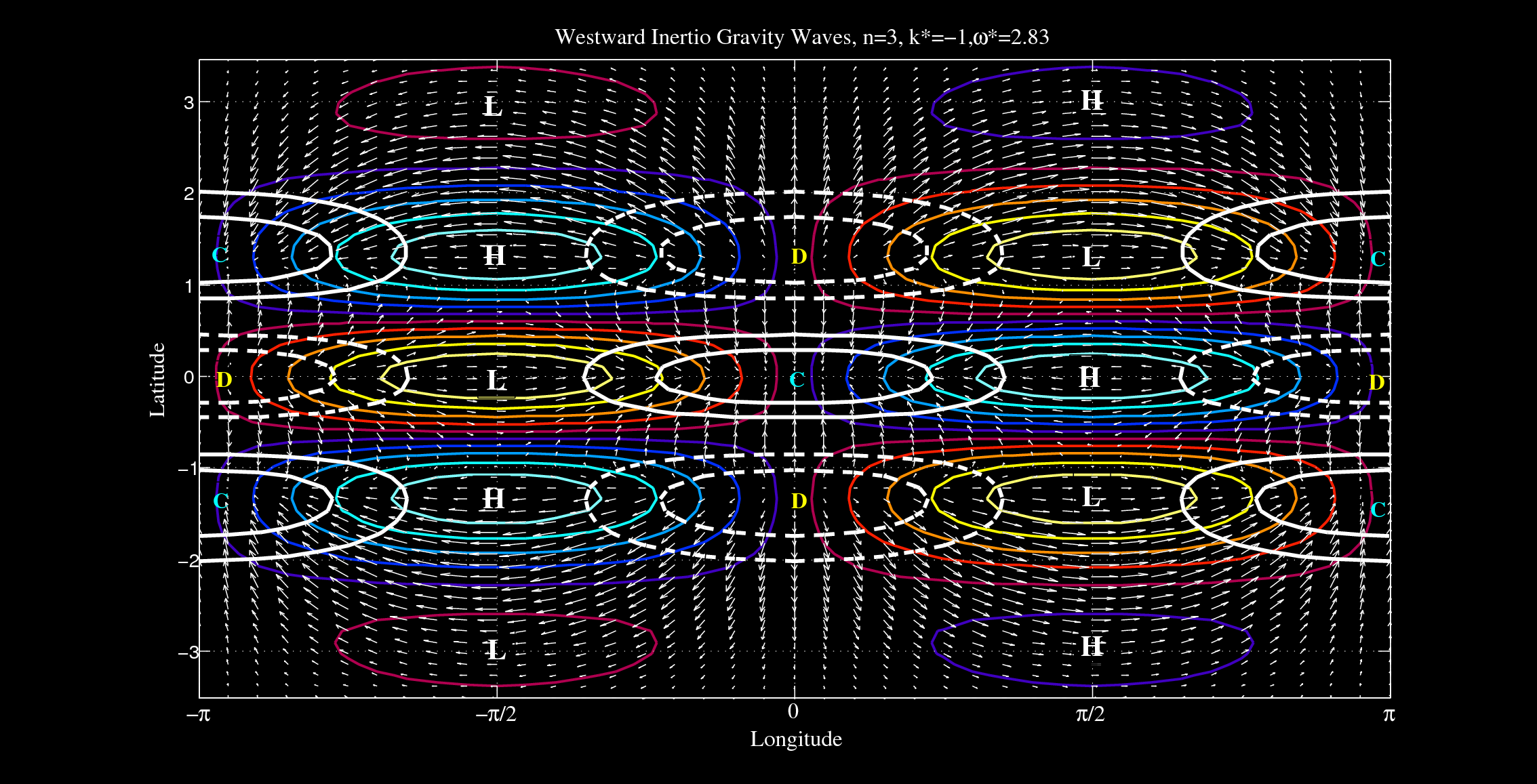
Theoretical structure of equatorially trapped waves of Matsuno’s normal modes superimposed with divergence and convergence of wind fields. All fields have been nondimensionalized by using the equatorial radius of deformation. Any further queries regarding the calculation can be found in this manuscript (part of my bachelor thesis): Sandro_Manuscript — [Click the button below to see my calculations related to equatorial waves and also the figure to see an animation related to cloud convective regions associated with Convergence Fields].
===

—
xxxx
“2D Theoretical Structures”
| >>ERn=1 | >> MRG n=0 | >> EIG=0 | >> EIGn=1 | >> WIGn=1 | >> Kelvin n=-1 |
| >>EIGn=2 | >> WIGn=2 | >> ERn=2 | >> EIGn=3 | >> WIGn=3 | >> ERn=3 |
xxx
“2D Theoretical Animations”
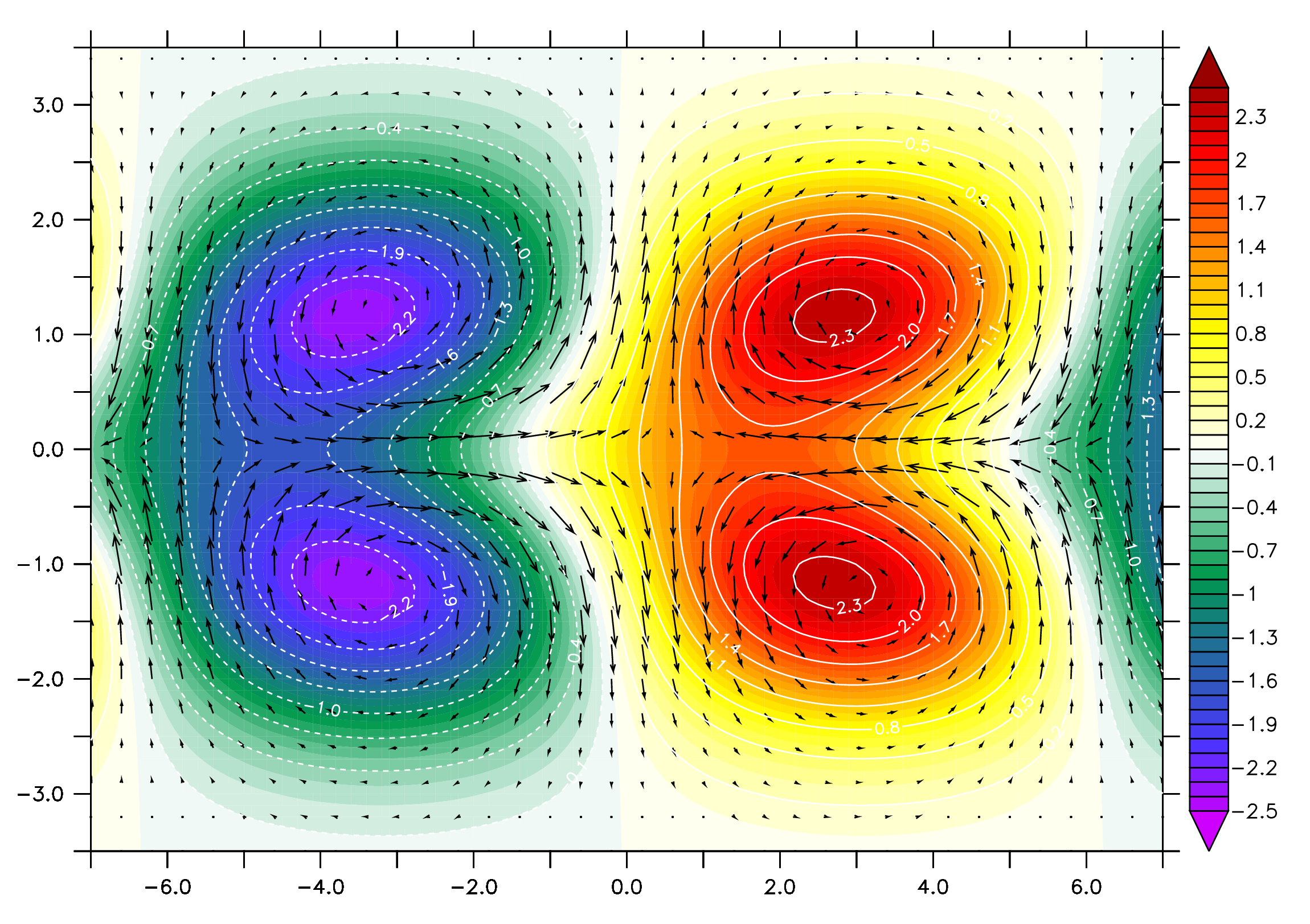
Animations of the Equatorially Trapped Waves of Matsuno’s normal modes superimposed with divergence and convergence of wind fields. The black solid lines indicate the convergence, while the divergence fields are represented by the dashed lines. Theoretical geopotential height structures are shown in color contours.
| >>Kelvin n=-1 | >> ERn=1 | >> EIGn=0 | >> MRG n=0 | >> EIGn=1 | >> WIGn=1 |
| >>EIGn=2 | >> WIGn=2 | >> ERn=2 | >> EIGn=3 | >> WIGn=3 | >> ERn=3 |

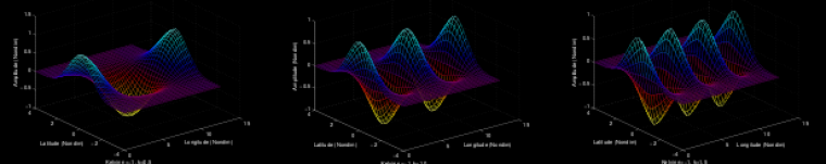
Equatorial Planetary Waves Amplitudes associated with Height perturbations for (a) Kelvin (Yellow), (b) MRG (red), (c) EIG n=0 (green), (d) Rossby waves n=1 (purple), (d) WIG n=1 (blue) and (e) WIG n=2 (white). All scales and fields have been nondimensionalized. X is nondimensionalized latitude and Y is amplitude.
==xxx==
“Observational Evidences”
“Convectively Coupled Equatorial Waves (CCEWs)”
======================================================
CCEWs play a crucial role in controlling the tropical weather system, as they modulate or organize the convection and a substantial portion of tropical rainfall and reinforce the tropical cyclone activities (e.g. Kiladis et al. 2009; Schreck et al. 2013, Kim and Alexander 2013 etc).
===
“2D Observational Variances of CCEWs”
Spatial distributions of the Filtered OLR variance 1981-2010 (30 years) for various parts of the wavenumber-frequency domain of interest. [All Season Variance]
| ERn=1 | MRG n=0 | Kelvin | EIGn=0 |
| WIGn=1 | WIGn=2 | TDD | MJO |
***
“2D Observational Snapshots in NCEPR2 & ERA”
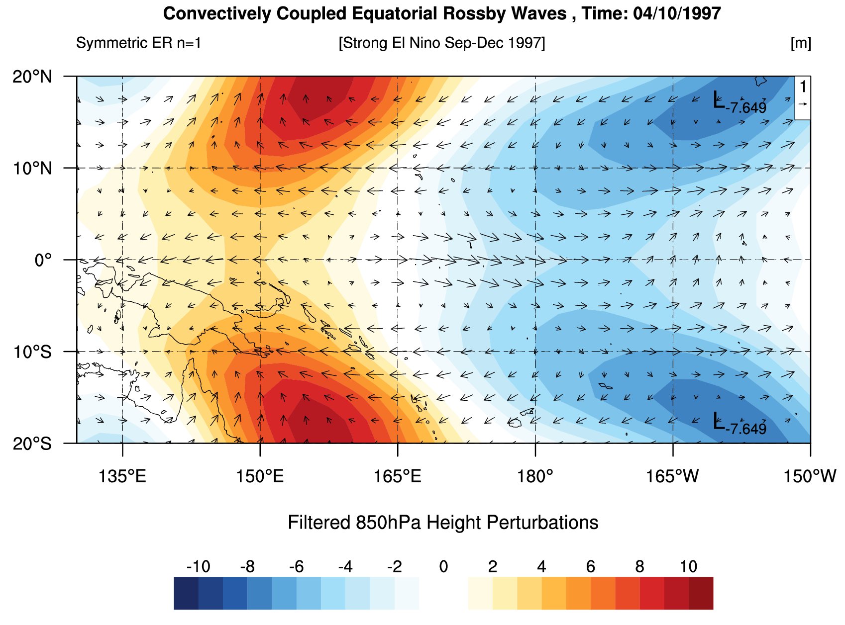
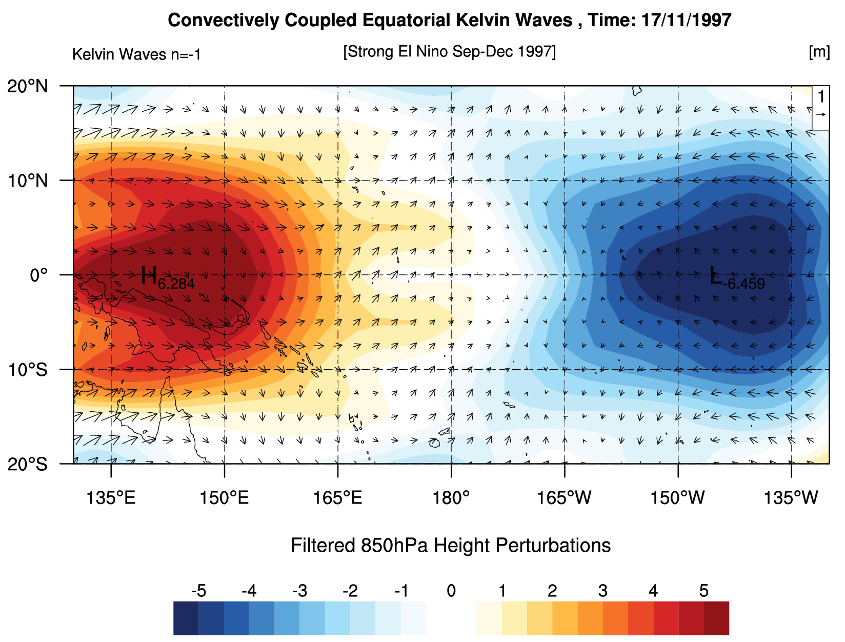
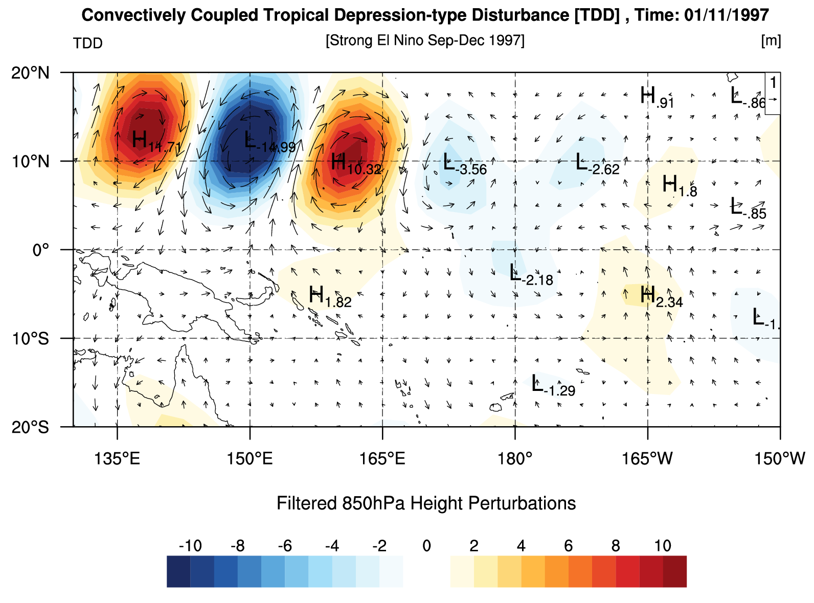
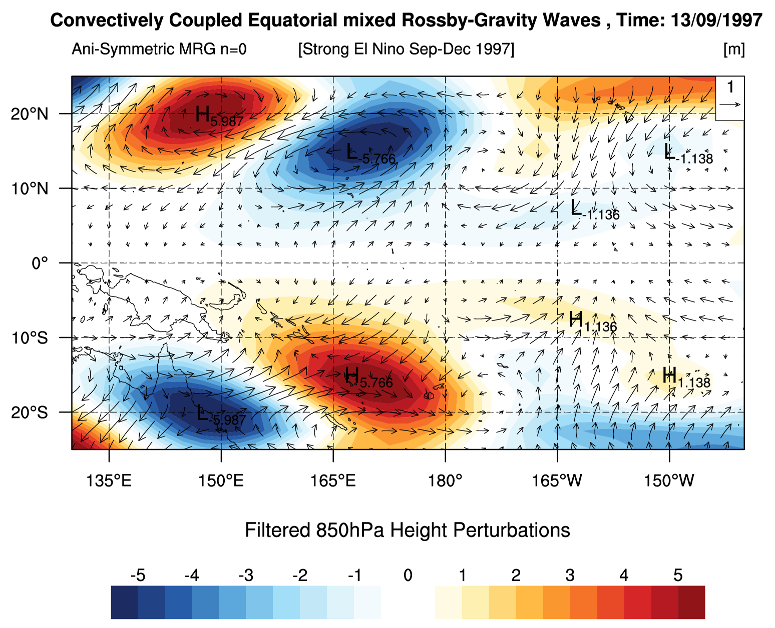
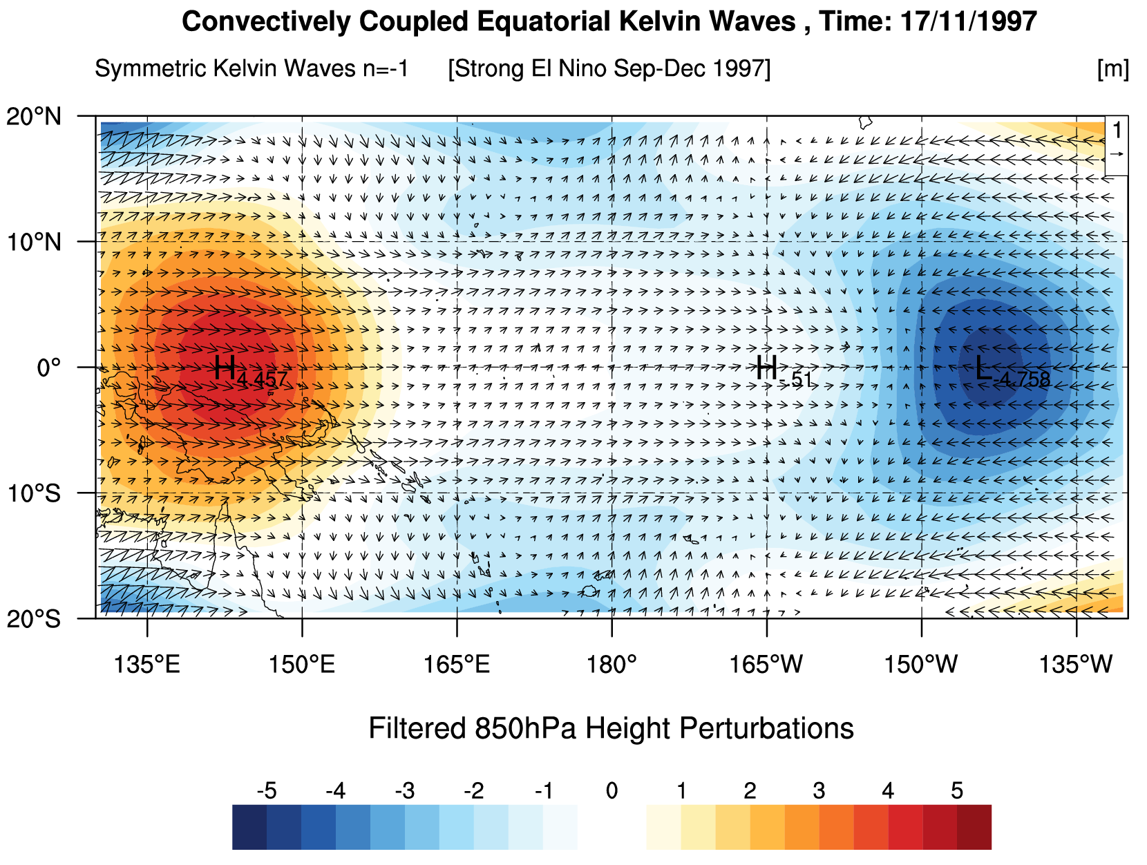
Snapshots and animations of the space-time filtered OLR assoaciated with CCEWs. Please kindly contact me for any further queries regarding the isolation technique. Reference vector is 1 m/s
NCEP-R2 [2.5 deg]
| ER Waves n=1 |
Kelvin Waves n=-1 |
TDD like-waves |
MRG waves n=0 |
ERA Interim – ECMWF [1.5 deg]
| ER Waves n=1 |
Kelvin Waves n=-1 |
TDD like-waves |
MRG waves n=0 |
XXX
===
“2D Animations of CCEWs in OLR, U, V, and Z”
**Filtered OLR Anomalies **
| Animations | Animations | Animations |
| MJO | Total Kelvin Waves n=-1 | Total ER Waves n=1 |
| Total MRG Waves n=0 | TDD/ Easterly Waves | Sym_Kelvin_Waves |
| Sym_ER_Waves | Anti_Sym_ER_Waves | Anti_Sym_MRG_Waves |
***
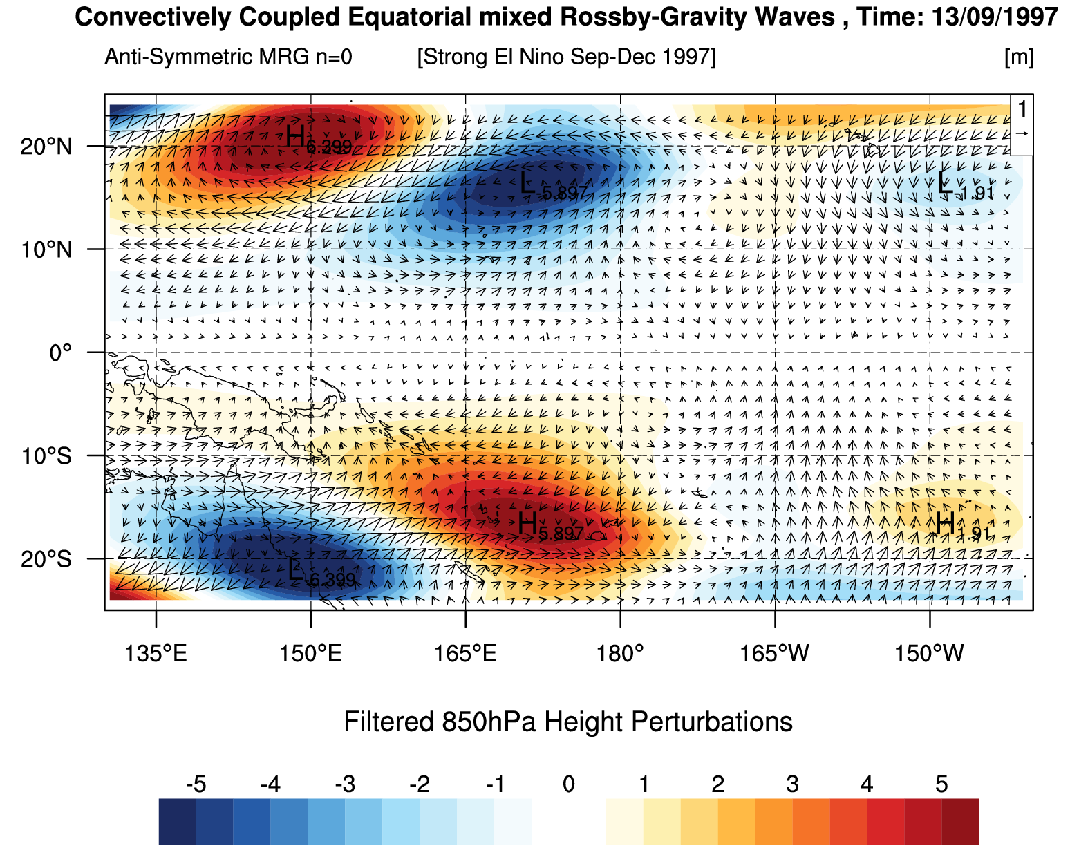
**Filtered OLR & 850 hPa Wind Perturbations**
| Animations | Animations | Animations |
| MJO | Total Kelvin Waves n=-1 | Total ER Waves n=1 |
| Total MRG Waves n=0 | TDD/ Easterly Waves | Sym_Kelvin_Waves |
| Sym_ER_Waves | Anti_Sym_ER_Waves | Anti_Sym_MRG_Waves |
***
**Filtered Geopotential Height & 850 hPa Wind Perturbations**
| Animations | Animations | Animations |
| MJO | Total Kelvin Waves n=-1 | Total ER Waves n=1 |
| Total MRG Waves n=0 | TDD/ Easterly Waves | Sym_Kelvin_Waves |
| Sym_ER_Waves | Anti_Sym_ER_Waves | Anti_Sym_MRG_Waves |
***
**Filtered Geopotential Height & 200 hPa Wind Perturbations**
| Animations | Animations | Animations |
| MJO |
Total Kelvin Waves n=-1 | Total ER Waves n=1 |
| Total MRG Waves n=0 | TDD/ Easterly Waves | Sym_Kelvin_Waves |
| Sym_ER_Waves | Anti_Sym_ER_Waves | Anti_Sym_MRG_Waves |
***
===== Spaca-Time Spectra Diagram (STSD) =====
****[Through Decomposition]****

****[Without Decomposition] ****
A. The Entire Calendar Years

===
B. Extended Summer and Winter
To find the dominant wave modes, the spectrum from each season is divided by the
annual mean of red noise (background).
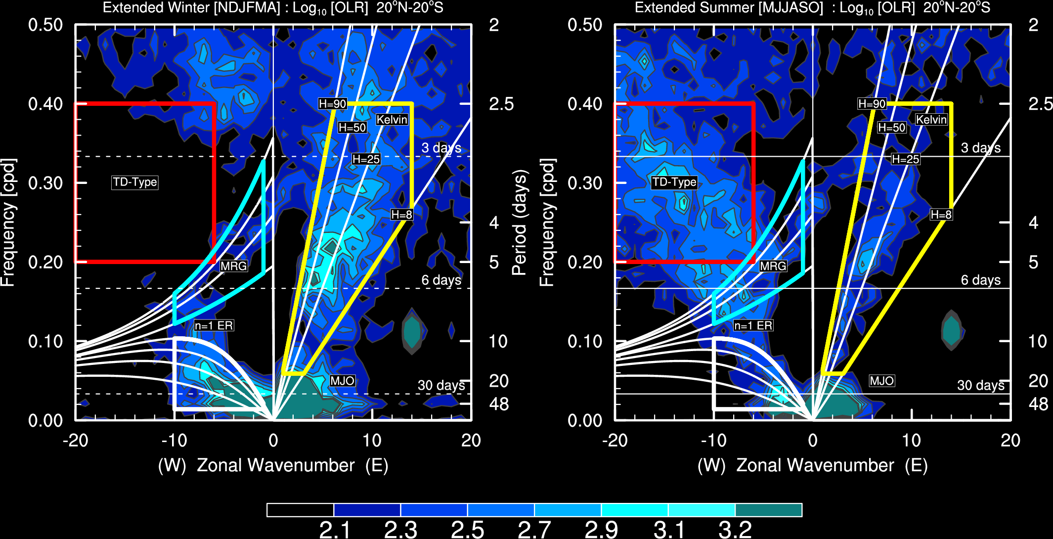
====
C. Seasonal Spectra
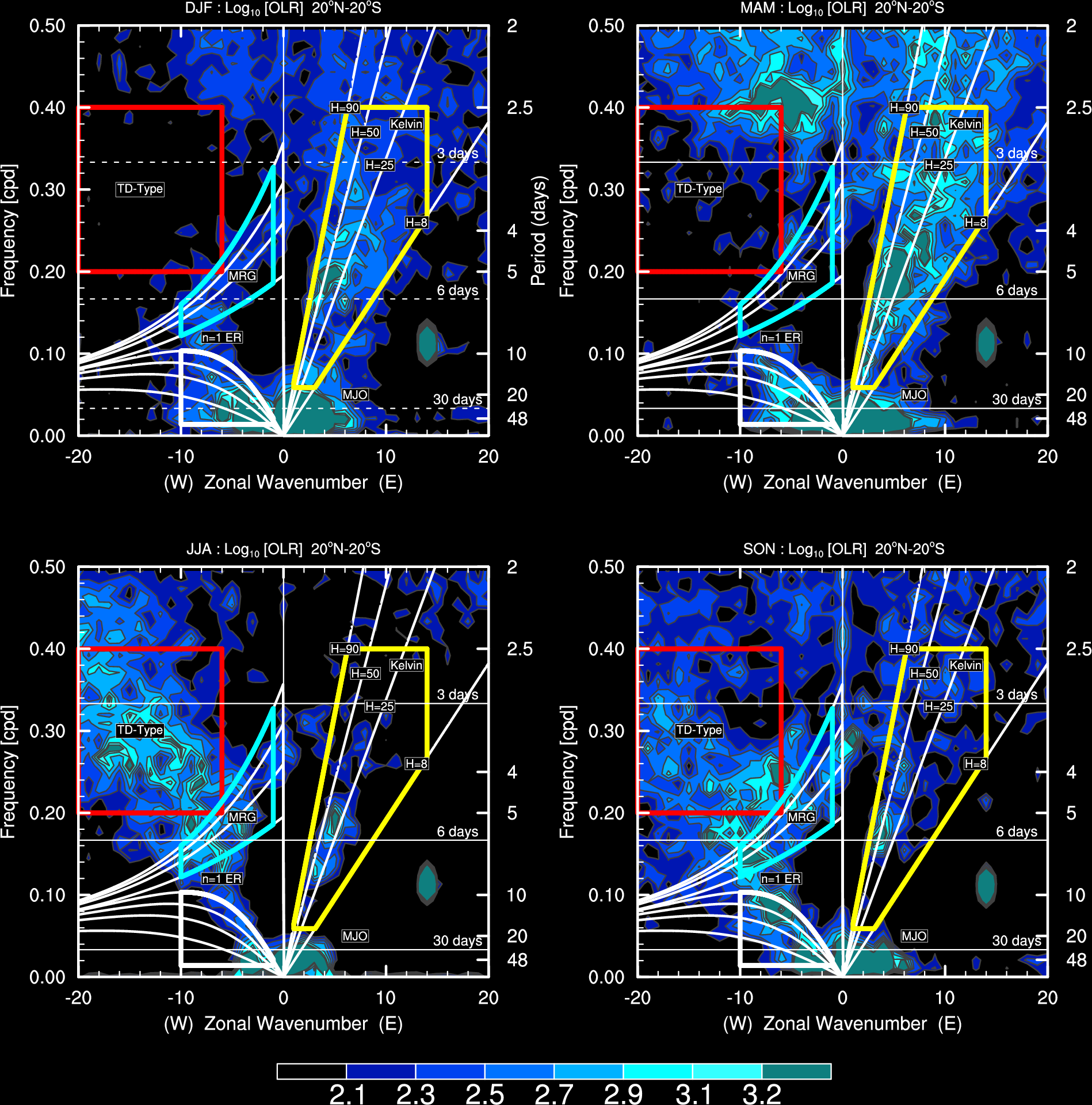
Note: Contour begins at a value of 2.1 for which the spectral signatures are statistically significantly above the background at the 95% level (based on 500 dof)– WK99.
===
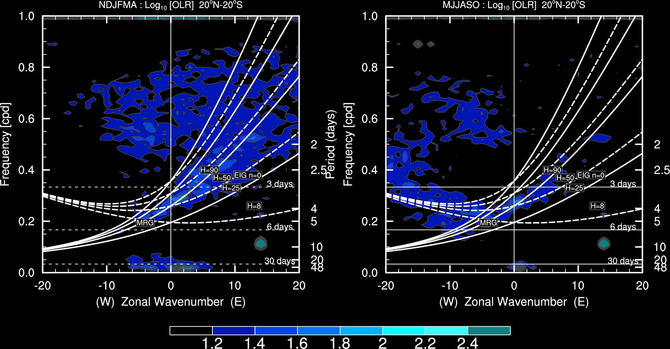
****[With Doppler Shifting Effect]****
XXX
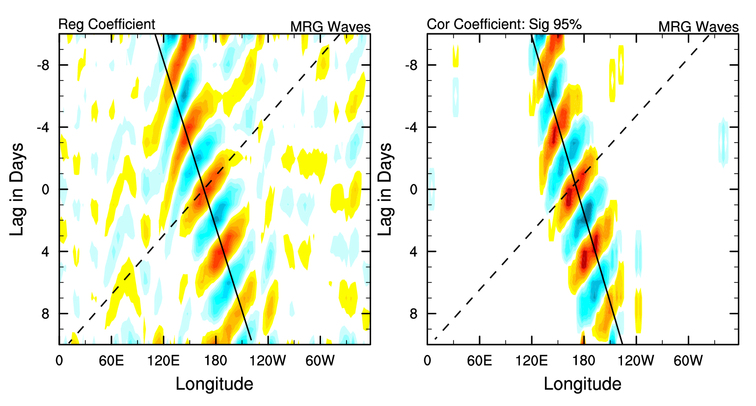
Composite Analysis of CCEWs in OLR
Hovmueller diagram of CCEWs. The OLR anomalies are regressed onto a time series of wave-filtered OLR anomalies (in this example: Kelvin, MRG, and ER waves).


===
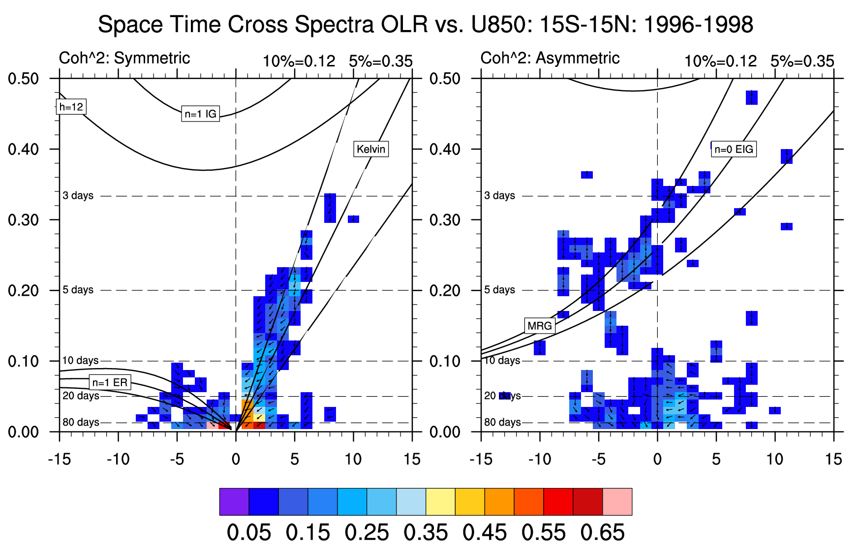
===== Spaca-Time Cross-Spectra Diagram (STCSD) =====
Space Time Cross Spectra OLR and Zonal Wind at 850 hPa level with a period of 96 days was chosen for the Fast Fourier Transform (FFT) with 65-day overlap and taper.

======================
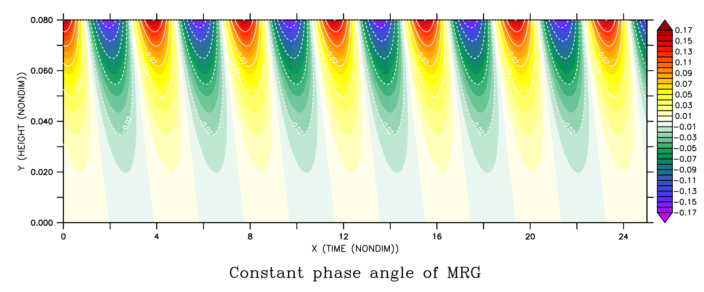
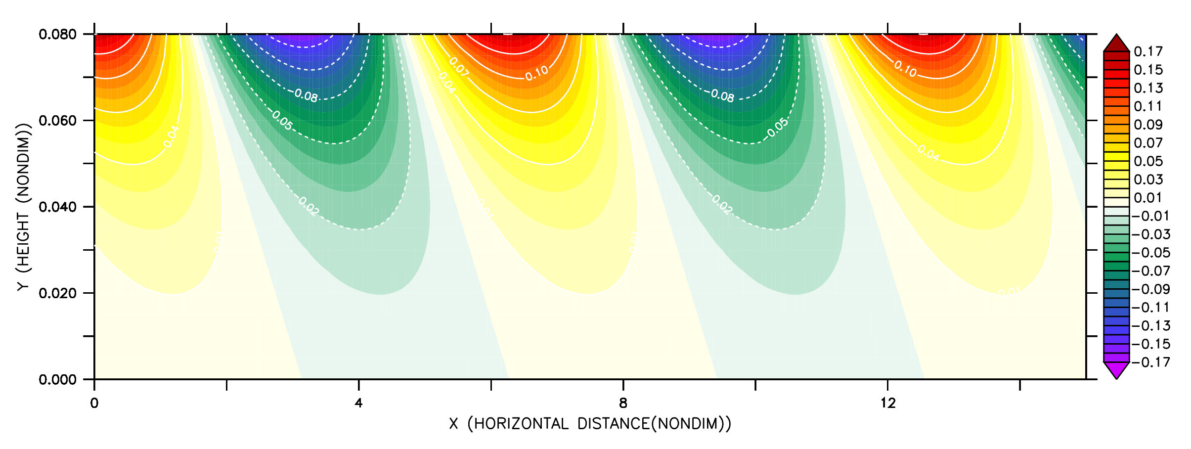
“Theory: Phase Angles of Kelvin and MRG Waves”
Constant Phase Angle of Kelvin Waves (n=-1) and MRG Waves (n=0)
Solving for particular “n” meridional wave mode number, we will find a set of frequency-vertical wavenumber relations for specific “n” that can reveal the slope of constant wave phase angle at the (Z,X) plane and at the (Z,t) plane in which Z is denoted as altitude, X is longitude, and t is time. The following figure is a vertical structure of free Kelvin waves and MRG n=0 in Z,X plane and Z,t plane in a constant N troposphere respectively, with Lz=6 km, he=10, H=7.3 km and dt/dz=-7 K/km. All units have been nondimensionalized using m* ≡ |m|β/Nk^2, ω* ≡ ωk/β, z*=z(Nk^2/β), t*=t(β/k), and x*=x/√(N/|m|β). The contours indicate the geopotential perturbations associated with the wave amplitude.


===============
Vertical Group Velocity of Kelvin Waves
Theoretical structure of vertical group velocity values (Cgz) for dry Kelvin waves in a constant N (Brunt–Väisälä frequency) troposphere and lower stratosphere with doppler shifting effect. Related articles: Kiladis et al. 2009 and Yang et al. 2011

===================
=====
The equatorial planetary waves (hereafter, EPW) are generated by diabatic heating due to organized tropical large-scale convective heating in the equatorial belt. Although they do not contain as much energy as other typical tropospheric weather disturbances, EPW causes predominant disturbances in the equatorial atmosphere, e.g., induces mean-meridional circulation, modulates the climatological cold tropopause, affects the patterns of low-level moisture convergence, controls the distribution of convective heating and convective storms in large longitudinal distances and also plays important role in the heat balance of the equatorial belt. Matsuno (1966) developed a model of quasi-geostrophic motions in the equatorial area to explain the characteristic of EPW by applying a single layer of a homogeneous incompressible fluid with free surface and assuming that Coriolis parameter to be proportional to the latitude. His work concerned with mathematical analyses of the simplified hydrodynamical equations, meanwhile Lindzen (1967) used the β-planes approximation and Laplace’s Tidal Equation to describe planetary waves in the equator and mid-latitudes. Both of these works are very fundamental to explain the main characteristic of equatorial planetary waves in the atmosphere.
A frequency-wavenumber spectral analysis technique has been performed to identify convectively coupled equatorial planetary waves (CCEWs) signals in the atmosphere using one of the proxies of tropical convection (in this case OLR) and other related variables such as geopotential height and wind velocity at 850 hPa and 200 hPa. The dispersion diagram was obtained by performing a two-dimensional space and time spectral analysis for 31 years. The wavenumber–frequency spectrum for unfiltered/filtered daily anomalies are divided by an estimate of the red background in order to normalize the data following Wheeler & Kiladis (1999, JAS) and Wheeler & Weickmann (2001, Monthly Weather Review) and then separated into a symmetric and anti-symmetric component. Data starts to cluster into different categories Kelvin waves, Mixed Rossby Gravity waves, Equatorial Rossby waves, TD-type waves, etc. It’s shown by spectral peaks tending to lie along the dispersion curves for shallow water equatorial waves (black lines) with flow background U=0. Should be noted in this case, anomalies are calculated from Smooth Daily Climatology by following this common procedure: (1) perform an FFT to get real and imaginary coefficients. (2) arbitrarily retain the 1st ‘nHarm’ coefficients. No change in coefficients. (3) set the (nHarm+1) real and imaginary coefficients to 0.5 of the original values. Set all others to 0.0. Presumably these are high-frequency noise. (4) Do a back transform with coefficients as described in (3). The procedure of filtering process for each wave meets the following criteria: MJO: Wave numbers 1to 5; period of 30-96 days, Kelvin waves: Wave numbers 1 to 14; period of 2.5-30 days; equivalent depth of 8-90m. ER waves: Wave numbers -1 to -10; period of 5-48 days; equivalent depth of 0-90m. MRG waves: Wave numbers -1 to -10; period of 3-10 days; equivalent depth of 8-90m. For each case, missing values are filled using linear interpolation in space and time. Contours are in a space-time filtered of the shaded field for each mode of the waves.
Horizontal Structure of CCEWs

Experiment 1. Equatorial Kelvin Waves period 2.5–17 days, wavenumber 1-14 and equivalent depth 8-90 m. Remarks: Propagation Direction is Eastward.

Experiment 2. Equatorially trapped Rossby waves period 9–72 days, wavenumber 1-10, and equivalent depth 0-90 m. Remarks: Propagation Direction is westward.

Experiment 3. Mixed Rossby-Gravity waves (MRG) period 3–10 days, wavenumber 1-10 and equivalent depth8-90 m. Remarks: Propagation Direction is westward.
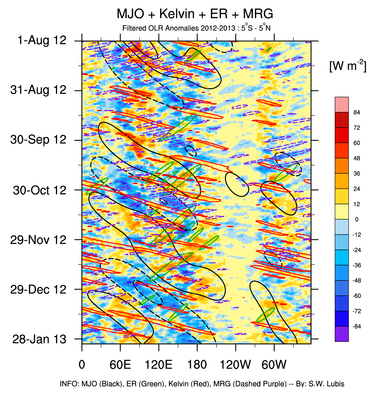
==Quartet Filter in Hovmöller Diagram==
Hovmöller Diagram of CCEWs using 2D FFT filters in space and time related to the time evolution of the waves in the average latitude. Contours are filtered in space-time. Data are first detrended and tapered in time, and filtered using a 2-dimensional fast Fourier transform (FFT). The procedure of filtering process for each wave follows these criteria: Kelvin Filtering: k= 1 to 14; period of 2.5-30 days; equivalent depth of 8-90m. MJO Filtering: k= 1 to 5; period of 30-96 days ER Filtering: k= -1 to -10; period of 5-48 days; equivalent depth of 8-90m. Black dashed lines indicate convectively active phases of MJO associated with negative anomalies of OLR.
==Dispersion Curves==
Theoretical dispersion curves (solid lines) are depicted for U=0 and separated into two components about the equator: symmetric and asymmetric


Figure 1. Wavenumber–frequency spectrum for unfiltered daily OLR and filtered anomalies of OLR [1980-2011, divided by an estimate of the red background following Wheeler & Kiladis (1999, JAS). The panel on the left shows signals that are anti-symmetric about the equator, while the panel on the right shows those that are symmetric. Spectral peaks tend to lie along the dispersion curves for shallow water equatorial waves (black lines). The unfiltered Omega shown above just to verify the constructed diagram that has been created.

Figure 2. Zonal wavenumber-frequency power spectra of the (a) antisymmetric component and (b) symmetric component of unfiltered daily OLR 1980-2011.

Figure 3. Zonal wavenumber-frequency spectrum of the base-10 logarithm of the ‘‘background’’ power calculated by averaging the individual power spectra of unfiltered daily OLR 1980-2011 in Figs. 2a and 2b, and smoothing many times with a 1-2-1.
Comparation to the Theoretical Structure of Tropical Waves
In this section, the two-dimensional structure of EPW based on the linear wave theory has experimented with specific frequency and modes. For details explanation please go directly to this article: Free Atmospheric Planetary Waves on an Equatorial β-plane Part I: Theoretical Background and Simulation. Simulation of horizontal wind and geopotential field perturbations corresponding to equatorial Rossby waves mode n= 1, which satisfies this general analytic solution:


Simulation of geopotential field and horizontal wind perturbations corresponding to Kelvin waves mode n= -1 with zonal wavenumber (k) =1.0 and Yanai waves mode n= 0 with zonal wavenumber (k)=1.0.

The theoretical dispersion relation for free equatorial planetary waves (EPW) in nondimensionalized wavenumber and frequency (Kelvin waves, Yanai waves, Rossby waves, East Poincare ́ waves (EIG) and West Poincare ́ waves (WIG).

–Sandro Lubis–
My special acknowledgment to Dr. Carl J. Schreck, III
===


