Tropical Dynamics and Equatorial Waves

Madden – Julian Oscillation (MJO) Part-I

•September 11, 2012 • 2 Comments

Filtering Techniques for Monitoring the Madden–Julian Oscillation

Reconstructed Codes by Sandro Lubis
Graduate Student of Leipzig Institute for Meteorology, University of Leipzig, Germany

All computations are made using
[ NCAR Command Language (NCL)]

September, 2012

In this experiment, Seasonal cycle is removed by subtracting the first three harmonics of the annual cycle. It is done by following this common procedure: (1) perform an FFT to get real and imaginary coefficients. (2) arbitrarily retain the 1st ‘nHarm’ coefficients. No change in coefficients. (3) set the (nHarm+1) real and imaginary coefficientsto 0.5 of the original values. Set all others to 0.0. Presumably these are high frequency noise. (4) Do a back transform with coefficients as described in (3) . In this case, anomalies are calculated from Smooth Daily Climatology. Annual cycle that contains more harmonics will more closely resemble the actual data. Data was retrieved OLR NOAA from 1980-2011. In order to obtain obvious phenomenon of MJO , filtering technique in time (20-100 days) and in space-time (k=1-5, 20-100d, Kiladis et all, 2009) are implemented. Missing values are linearly interpolated.

In order to test the reliability of the filter, the specific period was selected in which the phenomenon MJO was clearly visible. 2d FFT technique has been applied to see the direction of propagation of these oscillations.

Filter results in space and time (STSA) as well as in time (BPF) are shown in the panel diagram below. In general, both filters have almost the same capabilities in isolating OLR anomalies associated with the MJO phenomenon. Filters in space and time gives a smoother contour and more visible compared to the filter that only applied in time.

–Sandro Lubis–

Posted in Atmospheric Sciences (Meteorology and Climatolog)

Free Atmospheric Planetary Waves on an Equatorial β-plane Part I: Theoretical Background and Simulation

•August 2, 2012 • 1 Comment

Theoretical Simulation of Free Atmospheric Planetary Waves
on an Equatorial $\beta$ -plane

+Sandro Wellyanto Lubis and Sonni Setiawan
Department of Geophysics and Meteorology, Bogor Agricultural
University, Bogor 16680, Indonesia
+now in Leipzig Institute for Meteorology, University of Leipzig,
04103 Germany

All computations are made using
[ MATLAB – The Language of Technical Computing ]

2011

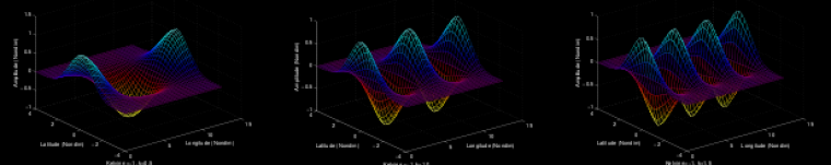
A simple theoretical model was developed to investigate behavior of equatorial planetary waves (EPW) on a motionless basic state of mean depth H on the equatorial barotropic $\beta$ -plane. Based on general nondimensional linearized equations of EPW in equatorial $\beta$ -plane, the amplitude of meridional wind perturbation (v’) is maximum at latitude y= $\pm$ 1 for mode n=1 and equal to zero at latitude y = ±1/2 $\sqrt{2}$ for mode n=2. The symmetric meridional wind perturbation (v’) with maximum amplitude at latitude y= ± 1 and antisymmetric zonal wind perturbation (u’) are some implications that correspond to simulation of Yanai waves in which the geopotential field perturbation ( $\Phi'$ ) is in the state of geostrophic balance at latitude -1< y <1 or – $(\beta^{-1}\sqrt{gH})^{1/2} > y > (\beta^{-1}\sqrt{gH})^{1/2}$ . The simulation of Kelvin waves resulted that either zonal wind or geopotential field has symmetric amplitude and symmetric perturbation relative to Earth’s latitude. Further filtered equatorial waves mode n=1, 2, and 3 showed that there are two classes of EPW which can be classified into high frequency Poincaré modes waves and the low frequency Rossby modes waves.

Figure 1. Simulation of geopotential field and horizontal wind perturbations corresponding to Yanai waves mode n= 0 with zonal wave number (k) = 0.5, =1.0, and 1.5, respectively (left panel) and Simulation of geopotential field and horizontal wind perturbations corresponding to Kelvin waves mode n= -1 with zonal wave number (k) =0.5, =1.0, and 1.5, respectively (right panel).

Figure 2. Simulation of horizontal wind and geopotential field perturbations corresponding to equatorial Rossby waves mode n= 1, 2, and 3.

Figrure 3. Simulation of horizontal wind and geopotential field perturbations corresponding to equatorial Eastward Poincaré waves mode n= 1, 2, and 3.

Figure 4. Simulation of horizontal wind and geopotential field perturbations corresponding to equatorial Westward Poincaré waves mode n= 1, 2, and 3.

Figure 5. Simulation of surface elevation corresponding to Kelvin waves, Yanai waves, Rossby waves, eastward Poincare waves and westward Poincare waves, respectively

Acknowledgements

**********************************************************************************
Sandro and Setiawan gladly acknowledge their gratefulness to Laurel McCoy
(Atmospheric Sciences, University of Missouri-Columbia, USA), Nina
Kargapolova (Institute of Computational Mathematics and Mathematical
Geophysics, Russia), and Davesh Vashishtha (University of Delhi, India) for
their contribution on reviewing this paper. The anonymous reviewers of this
paper provided valuable suggestions, and we truly appreciate them.

Posted in Applied Mathematics, Atmospheric Sciences (Meteorology and Climatolog)

QBO (Quasi-Biennial Oscillation) Part II

•July 29, 2012 • 1 Comment

QBO **(Quasi-biennial Oscillation)**

Analysis and Reconstructed Codes by Sandro Lubis
Graduate Student of Leipzig Institute for Meteorology, University of Leipzig, Germany

All computations are made using
[ NCAR Command Language (NCL) and Ferret NOAA]

July, 2012

Figure 1. Amplitude Spectrum and FFT Phase of QBO (Lubis, 2011)

Data: 1948-2011 NCEP Reanalysis I.

QBO or Quasi-Biennial Oscillation is indicated by zonally symmetric easterly and westerly wind regimes alternating regularly with periods varying from about 24-30 months in the equator. A simple analysis was conducted, zonal wind data from NCEP/NCAR Reanalysis [I] were directly used in order to identify the existence of QBO in the lower middle atmosphere during last decade (1948-2011). The chosen grid was located near the equator at 100 E and 2.5 N. The vertical average of zonal wind were computed due to an indication of the existence of QBO at 10-70 hPa. This result is consistent with previous studies (Dunkerton, 2003) show that alternating downward propagating westerly and easterly (E) regimes appear around the height of 10-70 hPa layer. Spectral analysis was applied to the average of zonal wind (10- 70hPa) from 1998-2010 giving the result that that the peak of spectral density is observed around 0.03-0.04 Hz month/cycle in other words the period of QBO cycle is obviously detected around 28 month/cycle. A 28 month/cycle is indicated by the max peak of amplitude as shown in figure. The maximum amplitude of QBO is 6.6 m/s and phase angle exceeds 160. The result of this spectral is realistic if it’s compared to the early study pointing out that QBO is associated to the alternating wind regimes repeating at intervals 22 to 34months, with an average period of slightly more than 28months (Baldwin et al., 2001, Holton and Matsuno 1984).

Figure 2. Zonal wind of QBO in period of 1948-2011 from NCEP/NCAR Reanalysis [I]

QBO (Quasi-Biennial Oscillation) Part I

-Sandro Lubis, Graduate student in Department of Meteorology, University of Leipzig, Germany, Germany 2011-

Posted in Atmospheric Sciences (Meteorology and Climatolog)

Mass Streamfunction

•June 17, 2012 • 1 Comment

Mass Streamfunction

Sandro Wellyanto Lubis,

Graduate Student of Leipzig Institute for Meteorology, University of Leipzig, Germany

[ All computations are made using NCAR Command Language (NCL)]

2012

Mass streamfunction $\Psi$ was computed using pressure coordinates from the ERA-Interim dataset 1989 – 2007. The streamfunction was determined by normalization of the inverse gravity and latitudinal belt using the equation of : $\frac{1}{acos\phi}\frac{\partial}{\partial\phi}\left(\left[\bar{v}\right]cos\phi\right)+\frac{\partial\bar{\omega}}{\partial p}=0$ . By defining the mass flux streamfunction $\Psi$ as the vertically integrated northward mass flux at latitude φ from pressure level p to the top of the atmosphere, the analytical solution for $\left [\bar{v}\right]$ can be obtained as $\frac{g}{2\pi acos\phi}\frac{\partial\psi}{\partial p}$ . Assumption that the streamfunction at the top of intergration is equal to zero, streamfunction $\Psi$ can be directly calculated from the observed $\left [\bar{v}\right]$ .

Figure 1. Zonal-mean cross section of the mass streamfunction in Tg/s for annual

In general, the mass streamfunction is commonly known as meridional overturning circulation (further, known as Hadley, Ferrel or polar cells depending on the latitudes) with unit 10^9 kg/s or Mt/s or Tg/s, the positive values (negative values) always denote to the clockwise (anticlockwise) rotation. The meridional overturning velocities are related to $\Psi$ by v and $\omega$ . There is a strong seasonal dependence of the streamfunction. In DJF, the rising motion is just south of the equator (in the southern or summer hemisphere) around 10S and sinks in the subtropics of NH around 30N. In JJA, the rising motion is fairly north of the equator, nearly at 20N and sinking in the subtropics of the SH, 30S. These shifted circulations are induced by the Asian summer monsoons and displacement of ITCZ. The strong upward motions occur on the summer hemisphere of equator where the huge covection and rising motion are intensively trigged by warm surface. Meanwhile, the strong downward air masses take place in the winter hemisphere of the equator. The annual mean (by averaging these values) produced two cells which are symmetric about the equator (the center is roughly around 5N). The center of these two symmetric cells denote the wet region in equator with high of cloud cover (further analysis using the OLR data).